Understanding and Implementing Simple Linear Regression from Scratch

Simple linear regression is often introduced with symbols and graphs that feel abstract, especially to learners encountering it for the first time. Yet at its core, it describes a pattern most people already understand from daily work and experience. The purpose of this article is to explain simple linear regression from the ground up, using concrete farming and agricultural analogies, and to show how the same idea later becomes a machine learning prediction method. By the end, the formula will feel less like mathematics and more like common sense written compactly.

The idea behind the equation

The equation of simple linear regression is written as y = c + m×x. Each symbol has a precise meaning, but the equation itself expresses a very ordinary idea: what you end up with equals what you already had plus what you gain (or lose) from doing some amount of work.

In this equation, y is the final outcome you care about, x is something you can observe or control, c is the starting amount before any action is taken, and m describes how much the outcome changes when x changes by one unit. Linear regression assumes that this change is consistent. Every additional unit of x changes y by the same amount.

A farming story for intuition

Imagine a wheat farmer at the start of the season. Before planting anything, the farmer already has some wheat stored in the barn from last year. That stored wheat is the starting point, which corresponds to c in the equation. Even if the farmer plants nothing this year, that wheat still exists.

Now consider the land being farmed. Each acre of land produces roughly the same amount of wheat if conditions are stable. The number of acres farmed is x, and the amount of wheat produced per acre is m. The total wheat after harvest, y, is simply the wheat that was already stored plus the wheat produced on each acre multiplied by the number of acres farmed.

Written in words, the equation says: total wheat equals stored wheat plus wheat per acre times acres farmed. Written mathematically, it becomes y = c + m×x. Nothing mysterious is happening; the equation is just a compressed description of the farming process.

Seeing the story as a graph

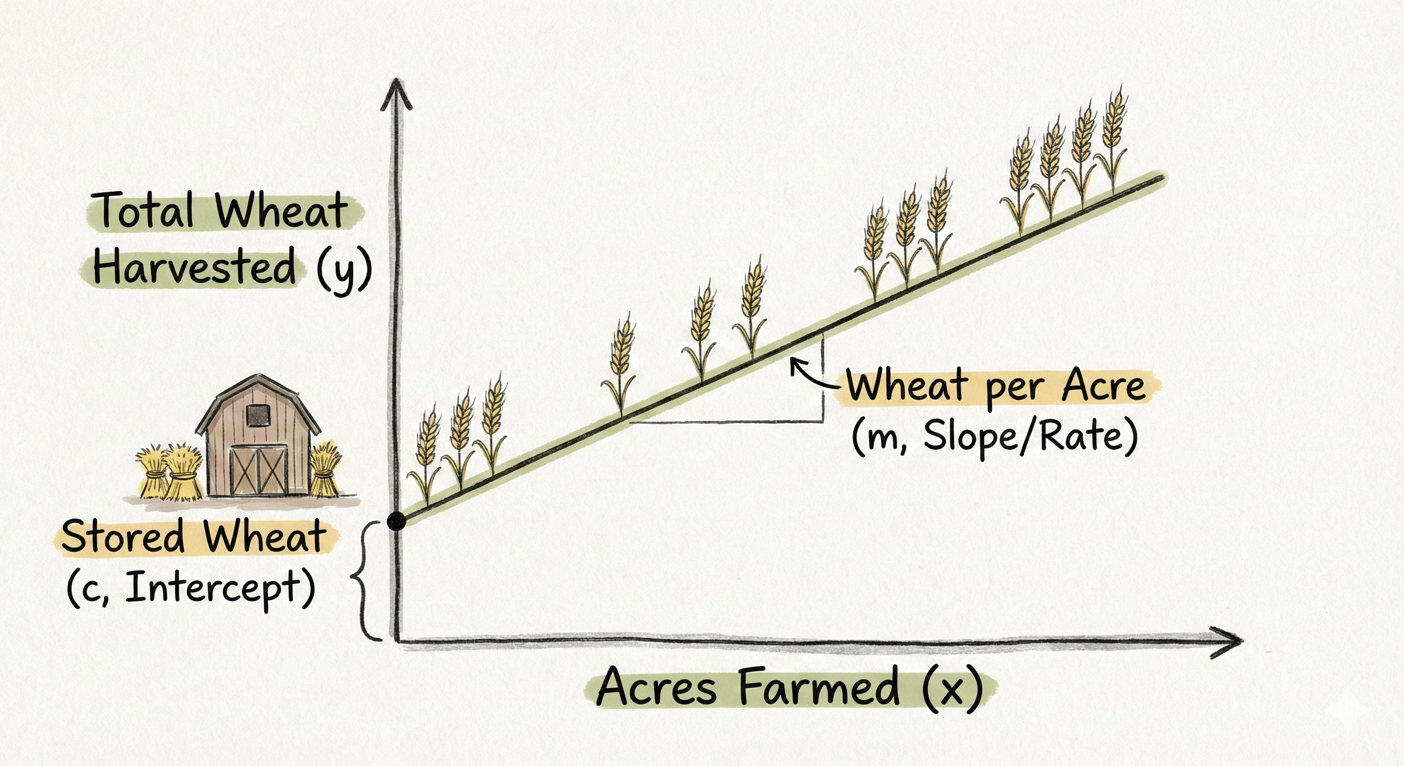
If this farming story is drawn on paper, the horizontal direction represents the number of acres farmed, and the vertical direction represents the total wheat at the end of the season. When zero acres are farmed, the graph does not start at zero wheat. It starts at the stored wheat in the barn. This starting height on the graph is the intercept, c.

As more acres are farmed, the total wheat increases steadily. Each extra acre adds the same amount of wheat, so the plotted points form a straight line. That straight line is the graphical version of the equation. It visually shows that the relationship between acres and total wheat is stable and predictable.

When more effort causes loss: negative slope

Not every season is good. Suppose the soil is poor, pests are rampant, or water is scarce. In such a case, each additional acre might cost more in seed and labor than it produces in harvest. Instead of gaining wheat by farming more land, the farmer loses wheat overall.

In the equation, this situation appears when m is negative. The starting wheat in the barn still exists, but every additional acre reduces the total. On the graph, the line slopes downward rather than upward. This negative slope does not mean the equation is wrong; it means the story it tells is one of diminishing returns or outright loss. Linear regression is neutral in this sense. It faithfully describes whether effort helps or hurts, as long as the change remains consistent.

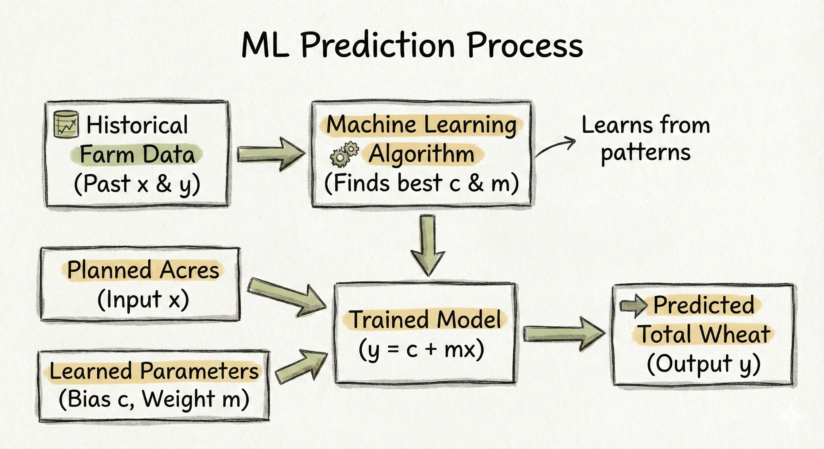
From farm records to prediction

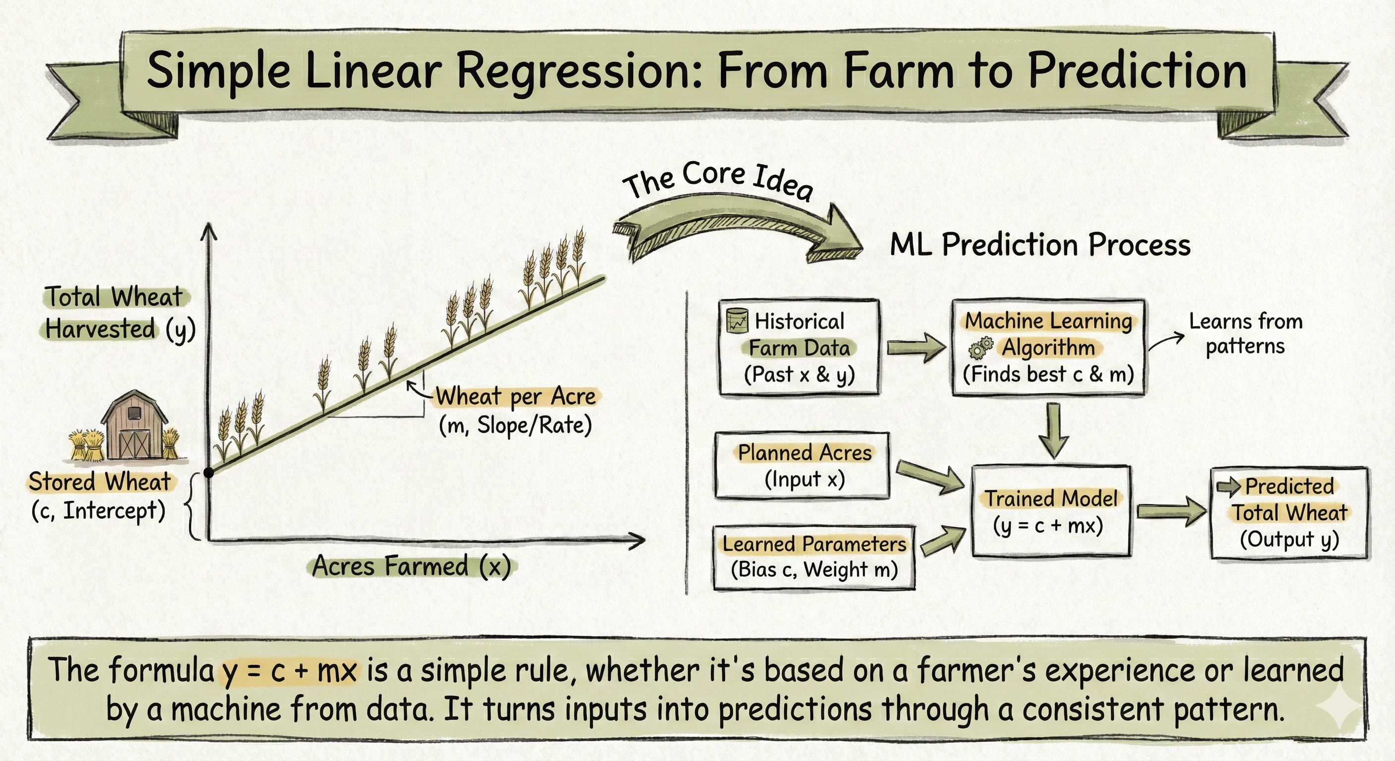
Now imagine the farmer has kept records for many years. For each year, the farmer wrote down how many acres were farmed and how much wheat was produced in total. Looking at this historical data, patterns begin to emerge. Years with more acres tend to have more wheat, or perhaps less wheat if conditions were bad.

This is where machine learning enters the picture. A simple linear regression model looks at past data and tries to find the best values of c and m that explain the observed relationship between x and y. Instead of the farmer choosing these values based on intuition, the computer estimates them from data.

Once c and m are learned, the equation can be used for prediction. Given a planned number of acres for the coming season, the model can estimate the expected total wheat. In machine learning terms, x is an input feature, y is the predicted output, c is the bias or intercept, and m is the learned weight. Conceptually, however, it is still the same farming story.

The same pattern with milk, cows, rain, and fertilizer

The same equation appears in many agricultural settings. Consider a dairy farmer who starts the day with some milk already stored in cooling tanks. Each cow produces roughly the same amount of milk per day. The total milk at the end of the day equals the stored milk plus milk per cow times the number of cows milked.

Or consider soil nutrients. The soil already contains some nutrients at the start of the season. Each bag of fertilizer adds a fixed amount. The final nutrient level equals the initial level plus nutrients per bag times the number of bags applied. In each case, the structure of the relationship is identical. There is a starting point and a steady change per unit of action.

Why “linear” matters

The word “linear” is important because it encodes a strong assumption: consistency. Linear regression assumes that each additional unit of x changes y by the same amount, regardless of how large x already is. This is why the graph is a straight line and why the equation remains simple.

In real life, many processes eventually stop being linear. Land can become saturated, cows can only produce so much milk, and fertilizer can damage crops beyond a certain point. Simple linear regression does not capture those complexities. Its value lies in being the simplest useful model, one that is easy to understand, easy to compute, and often good enough for first approximations.

Closing perspective

Simple linear regression is not just a statistical technique; it is a formal way of expressing a very old human habit: starting with what we have and estimating how outcomes change with effort. The equation y = c + m×x is powerful precisely because it is humble. It turns experience into a rule, a rule into a line, and a line into a prediction. When understood through concrete stories like farming, its logic becomes intuitive, and its later role in machine learning feels like a natural extension rather than a leap into abstraction.